How to Use the Empirical Rule on a Calculator: Step-by-Step Guide to Mastering This Tool
The empirical rule, or 68-95-99.7 rule, is a powerful statistical tool for understanding data in a normal distribution. Using an empirical rule calculator simplifies applying this rule to real-world data, like test scores or heights, by quickly calculating the percentage of data within one, two, or three standard deviations of the mean. This guide walks you through how to use the calculator effectively, with clear steps, examples, and tips. Whether you’re a student, teacher, or data enthusiast, you’ll master this tool in no time. For a deeper dive into the rule itself, check out our guide on what the empirical rule is.
What Is an Empirical Rule Calculator?
An empirical rule calculator is an online tool that automates calculations for the 68-95-99.7 rule. It takes your data’s mean (μ) and standard deviation (σ) and computes the percentage of data within specific ranges or probabilities for a given value. This saves time and reduces errors, especially for complex datasets. The calculator is ideal for analyzing normally distributed data, such as exam grades or biological measurements, and is perfect for beginners and experts alike.
Why Use an Empirical Rule Calculator?
Here’s why an empirical rule calculator is a game-changer:
Speed: Get instant results without manual calculations.
Accuracy: Avoid errors in computing standard deviations or percentages.
Ease: Input simple values (mean, standard deviation, range) for quick insights.
Learning: Understand the 68-95-99.7 rule through practical application.
Ready to try it? You can use our calculator to follow along with the steps below.
Step-by-Step Guide to Using the Empirical Rule Calculator
Follow these steps to use an empirical rule calculator effectively. We’ll include an example to make it crystal clear.
Step 1: Gather Your Data
Identify the mean (average) and standard deviation of your dataset. These are the key inputs for the calculator.
Example: Suppose you’re analyzing exam scores with a mean of 75 and a standard deviation of 10. You want to know what percentage of students scored between 65 and 85.
Step 2: Input the Mean and Standard Deviation
Enter the mean (μ = 75) and standard deviation (σ = 10) into the calculator’s fields. Most calculators also let you specify a range or a specific value for analysis.
Step 3: Define the Range or Value
For a range, input the lower and upper bounds (e.g., 65 and 85). For a specific value, enter the score you’re analyzing (e.g., 80). In our example, we’ll use the range 65 to 85.
Step 4: Select the Calculation Type
Choose what you want to calculate:
Percentage within a range: Find the proportion of data between two values (e.g., 65 to 85).
Probability for a value: Determine the likelihood of a score being below or above a specific value.
Percentile: Find the percentile rank of a value in the distribution.
For our example, select “percentage within a range” for 65 to 85.
Step 5: Interpret the Results
The calculator applies the empirical rule (68%, 95%, 99.7%) to your inputs. For our example:
The range 65 to 85 is 75 ± 10, or μ ± 1σ.
The empirical rule says 68% of data falls within one standard deviation.
Result: Approximately 68% of students scored between 65 and 85.
Some calculators also provide Z-scores for precision. For instance, a score of 80 has a Z-score of (80 – 75) / 10 = 0.5, which you can use with a Z-table for exact probabilities.
Step 6: Verify and Apply
Double-check your inputs for accuracy. Use the results to make decisions, like predicting student performance or setting benchmarks. If the data isn’t normally distributed, the calculator may flag this or suggest alternative methods.

Real-World Example: Applying the Calculator
Let’s try another example to solidify your understanding.
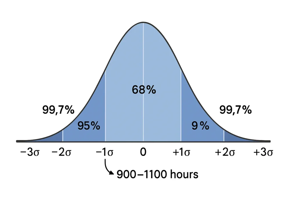
Scenario: A factory produces light bulbs with a mean lifespan of 1000 hours and a standard deviation of 100 hours. You want to know the percentage of bulbs lasting between 900 and 1100 hours.
Input Data: Enter mean = 1000, standard deviation = 100.
Set Range: Input 900 to 1100 hours.
Calculate: The calculator recognizes 900 to 1100 as μ ± 1σ, so 68% of bulbs last within this range.
Result: Approximately 68% of bulbs have lifespans between 900 and 1100 hours.
This helps the factory predict inventory needs or warranty claims. The calculator makes this process fast and error-free.
Tips for Using the Empirical Rule Calculator
Check Normality: Ensure your data is approximately normal (bell-shaped) using a histogram or normality test. The empirical rule doesn’t work for skewed data.
Use Precise Inputs: Accurate mean and standard deviation values ensure reliable results.
Explore Features: Some calculators offer graphs or Z-score options for deeper analysis.
Cross-Check: For critical decisions, verify results with manual calculations or a Z-table.
Did You Know? The empirical rule is an approximation. For precise probabilities, especially outside the 68-95-99.7 ranges, consider using a Z-score calculator.
Common Mistakes to Avoid
Non-Normal Data: Applying the rule to skewed or bimodal data leads to inaccurate results.
Incorrect Inputs: Mixing up mean and standard deviation or entering wrong values can skew outputs.
Misinterpreting Ranges: Ensure your range aligns with standard deviation intervals (e.g., ±1σ, ±2σ).
Ignoring Sample Size: Small datasets (under 30) may not be normally distributed, reducing accuracy.
When to Use the Empirical Rule Calculator
The calculator is perfect for:
Students: Simplifying homework or exam prep for statistics courses.
Teachers: Demonstrating the empirical rule with real data.
Analysts: Quickly estimating probabilities in fields like finance or quality control.
Researchers: Analyzing normally distributed data, like biological measurements.
It works best when your data forms a bell-shaped curve. If your data is skewed, consider tools like Chebyshev’s Theorem for broader applicability.
Frequently Asked Questions (FAQs)
It uses the 68-95-99.7 rule to calculate the percentage of data within one, two, or three standard deviations of the mean based on your inputs.
You need the mean and standard deviation of your dataset, plus a range or specific value to analyze.
No, the empirical rule only applies to normal distributions. For non-normal data, use other statistical methods.
The empirical rule gives specific percentages (68%, 95%, 99.7%) for normal distributions. Chebyshev’s Theorem applies to any distribution but offers less precise estimates, like at least 75% within two standard deviations.
It’s accurate for approximately normal data but is an approximation. For precise results, pair it with Z-score calculations.
A calculator saves time, reduces errors, and often includes visualizations to help you understand the results.
Conclusion
Using an empirical rule calculator makes mastering the 68-95-99.7 rule a breeze. By inputting your data’s mean, standard deviation, and range, you can quickly find percentages or probabilities in a normal distribution, whether you’re analyzing exam scores, product lifespans, or biological data. This step-by-step guide equips you to use the tool confidently, avoiding common pitfalls and applying it to real-world scenarios. Ready to crunch your numbers? Use our calculator to simplify your analysis and explore the empirical rule’s power. For foundational knowledge, learn more about what the empirical rule is to deepen your understanding.
Other Resources:
- What Is the Empirical Rule: A detailed explanation of the 68‑95‑99.7 rule.
- Empirical Rule vs. Chebyshev’s Theorem: Compare these statistical tools for better analysis.
- Applications of the Empirical Rule in Statistics and Probability: Discover real‑world uses.
- Normal Distribution and the Empirical Rule: Comprehensive insights into normal distributions.
- All Tools: Browse our full collection of statistical calculators.