Empirical Rule vs. Chebyshev’s Theorem: Compare These Statistical Tools for Better Analysis

When analyzing data distributions, two statistical tools stand out: the empirical rule and Chebyshev’s theorem. Both help estimate how data spreads around the mean, but they differ in scope, precision, and application. The empirical rule, also called the 68-95-99.7 rule, is tailored for normal distributions, while Chebyshev’s theorem applies to any dataset, offering broader but less specific insights. This guide compares these tools, highlighting their differences, strengths, and real-world uses to help students, analysts, and researchers choose the right one. Curious to try the empirical rule? You can test it now with a dedicated tool.

What Is the Empirical Rule?

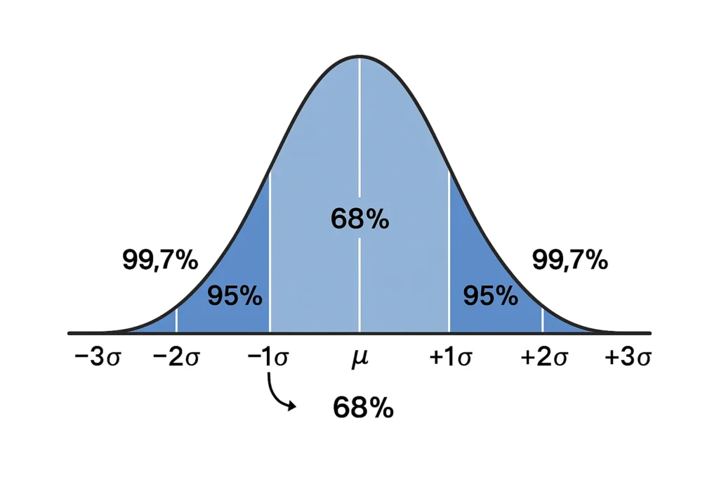
The empirical rule applies to normal distributions, which form a bell-shaped curve. It states:

68% of data lies within one standard deviation (σ) of the mean (μ).
95% of data is within two standard deviations.
99.7% of data falls within three standard deviations.

This rule is precise because it’s designed for datasets that are symmetric and bell-shaped, like test scores or heights. It’s a quick way to estimate probabilities and data spread in fields like education or quality control.

What Is Chebyshev’s Theorem?

Chebyshev’s theorem is a universal tool that applies to any data distribution, regardless of shape—normal, skewed, or otherwise. It provides a minimum percentage of data within a certain number of standard deviations from the mean, calculated as:

At least 1 – 1/k² of data lies within k standard deviations of the mean (where k > 1).

For example:

For k = 2 (two standard deviations), at least 1 – 1/2² = 75% of data is within ±2σ.
For k = 3, at least 1 – 1/3² ≈ 88.89% of data is within ±3σ.

This makes Chebyshev’s theorem versatile but less precise than the empirical rule for normal data.

Key Differences Between Empirical Rule and Chebyshev’s Theorem

Here’s a side-by-side comparison to clarify their differences:

Feature	Empirical Rule	Chebyshev’s Theorem
Applies To	Normal distributions only	Any distribution (normal or not)
Percentages	68%, 95%, 99.7% for ±1σ, ±2σ, ±3σ	At least 1 – 1/k² for k > 1
Precision	Specific and precise	Minimum estimates, less precise
Use Case	Quick estimates for bell-shaped data	Broad analysis for any dataset
Example Output	95% within ±2σ	At least 75% within ±2σ

The empirical rule shines for its accuracy in normal distributions, while Chebyshev’s theorem is a fallback for non-normal data, like skewed financial datasets.

When to Use Each Tool

Empirical Rule

Use the empirical rule when:

Your data is approximately normal (bell-shaped, symmetric).
You need precise percentages (68%, 95%, 99.7%).
You’re analyzing data like test scores, heights, or IQs.

Example: For SAT scores with a mean of 1000 and a standard deviation of 150, the empirical rule predicts 95% of scores fall between 700 and 1300. You can test it now to see this in action.

Chebyshev’s Theorem

Use Chebyshev’s theorem when:

Your data is not normal (e.g., skewed, bimodal, or irregular).
You need a conservative estimate of data spread.
You’re working with small or uncertain datasets.

Example: For customer wait times (skewed data) with a mean of 20 minutes and a standard deviation of 5 minutes, Chebyshev’s theorem guarantees at least 75% of wait times are between 10 and 30 minutes.

Real-World Examples

Example 1: Test Scores (Empirical Rule)

A class’s math scores are normally distributed with a mean of 80 and a standard deviation of 8. Using the empirical rule:

68% of students score between 72 and 88.
95% score between 64 and 96.
99.7% score between 56 and 104.

This helps teachers identify typical performance ranges. For more practical applications, explore real-world uses.

Example 2: Delivery Times (Chebyshev’s Theorem)

A delivery service’s times are skewed, with a mean of 45 minutes and a standard deviation of 10 minutes. Chebyshev’s theorem says:

At least 75% of deliveries take 25 to 65 minutes (±2σ).
At least 88.89% take 15 to 75 minutes (±3σ).

This conservative estimate helps plan logistics for non-normal data.

Limitations of Each Tool

Empirical Rule Limitations

Normal Data Only: Fails for skewed or non-normal distributions.
Sample Size: Needs large samples (30+) to ensure normality.
Approximation: Assumes perfect normality, which real data may not fully meet.

Chebyshev’s Theorem Limitations

Less Precise: Provides minimum percentages, not exact ones.
Conservative: May underestimate data concentration in normal distributions.
Complex Calculation: Requires computing 1 – 1/k² for each k value.

Which Tool Should You Choose?

Choose the Empirical Rule for normally distributed data when you need specific, reliable percentages. It’s ideal for education, biology, or quality control where bell-shaped curves are common.
Choose Chebyshev’s Theorem for non-normal or unknown distributions, like financial data or irregular measurements, when you need a safe, broad estimate.

Did You Know? Combining both tools can enhance analysis. Use the empirical rule for normal data and Chebyshev’s theorem as a fallback for uncertain datasets.

Frequently Asked Questions (FAQs)

What is the difference between Chebyshev’s theorem and the empirical rule?

The empirical rule applies to normal distributions with fixed percentages (68%, 95%, 99.7%). Chebyshev’s theorem works for any distribution, giving minimum percentages (e.g., at least 75% within ±2σ).

When should I use the empirical rule calculator?

Use it for normally distributed data, like test scores or heights, to calculate precise percentages within standard deviation ranges.

Can Chebyshev’s theorem be used for normal distributions?

Yes, but it’s less precise, offering minimum percentages (e.g., at least 75% vs. 95% for ±2σ).

Why is the empirical rule more precise?

It’s designed for normal distributions, which have predictable patterns, unlike Chebyshev’s theorem, which applies broadly.

What types of data suit Chebyshev’s theorem?

Skewed, bimodal, or any non-normal data, like income or wait times, where normality isn’t guaranteed.

Conclusion

The empirical rule and Chebyshev’s theorem are essential for analyzing data spread, but they serve different needs. The empirical rule offers precise percentages (68%, 95%, 99.7%) for normal distributions, perfect for bell-shaped data like test scores. Chebyshev’s theorem provides flexible, conservative estimates for any dataset, ideal for skewed or irregular data. Understanding their differences helps you pick the right tool for your analysis. Try test it now to see the empirical rule in action, or explore real-world uses for practical applications.